Digital Audio Effects Processing with Csound

Digital Audio Primer

This digital audio primer provides step-by-step instructions on setting up a development platform for audio effects processing.

Recording with Audacity
Csound
Wave File Format
Analog to Digital Conversion
Digital to Analog Conversion
References

Audacity is audio editing software that facilitates the recording, playback, importing and exporting of audio files. It is free, easy to use, and available for Windows, Mac, and Linux operating systems. When recording audio data, Audacity allows the user to specify four necessary parameters to successfully import this data into Csound – file format, sampling rate, sample size, and number of channels.

1. Getting Audacity

Go to the Audacity home page - http://audacity.sourceforge.net/

Download and install Audacity version 1.2.1 for the appropriate operating system. Tutorials, detailed instructions, an FAQ, and online help are all available from the same page.

2. Set the recording preferences

Select preferences from the file menu

Set the number of channels

Set the sampling rate

Set sample size

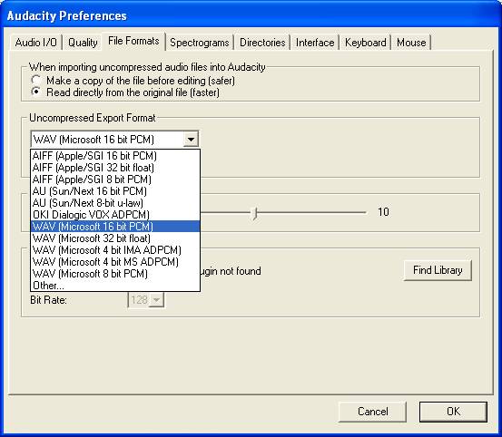
Set file format

3. Record your track – detailed instructions are available from the help menu

4. Export your track as a wave file - you now have an unprocessed wave file ready to be imported into Csound

Select “Export as WAV…”

Top

Csound

Like Audacity, Csound is multi-platform freeware. Csound renders audio data according to the text-based instructions of two interdependent and complimentary text files – the orchestra file (.orc) and the score (.sco) file. Conveniently, the two files can be combined into one Csound file (.csd). The complete list of commands with detailed syntax is available from the Public Csound Manual - http://www.lakewoodsound.com/csound/hypertext/manual.htm

1. Getting Csound

Go to the Csound FrontPage - http://mitpress.mit.edu/e-books/csound/frontpage.html

Download and install Csound version 4.23 for the appropriate operating system. Tutorials, detailed instructions, an FAQ, and online help are all available from the same page.

2. Running Csound

Running the executable file created in the installation process will bring up the following command window:

- Set the path of the orchestra file (.orc) or Csound file (.csd) in the first text box

- Set the path of the score file (.sco) in the second text box

- Set the path of the output file in the third text box

- Select the file format in the ‘Format’ panel

- Set the sample size in the ‘Size’ panel

- Make sure the file format and sample size match the recording preferences set in Audacity

- Click the ‘Render’ button to execute the procedure

3. The Orchestra File

The orchestra file is divided into two separate sections – the header section and the instrument section.

a. The Header Section

This section defines four parameters – sample rate (sr), control rate (kr), the sampling rate divided by the control rate (ksmps) and the number of channels (nchnls). The sampling rate and number of channels must match the recording preferences set in Audacity. The following code fragment is the header from an orchestra file:

sr = 48000

kr = 4800

ksmps = 10

nchnls = 2

b. The Instrument Section

The instrument section is composed, appropriately, of a series of instruments. However, these are not instruments in the traditional sense. Each instrument is a function made up of interconnecting modules (opcodes) that generate or modify signals based on specified parameters. These opcodes are processed top to bottom left to right. The following code reads the left and right channels of a stereo track called ‘audio_file.wav’ and plays them aloud:

instr 1
ar1, ar2 soundin "audio_file.wav"
outc ar1, ar2
endin

This can be parsed line by line to determine exactly how it works.

instr 1

This line declares that a new instrument referenced by the number 1 is being defined by the subsequent code.

ar1, ar2 soundin "audio_file.wav"

The ‘soundin’ opcode reads the two channels of the audio file ‘audio_file.wav’ and stores them in two separate signals, ‘ar1’ and ‘ar2’. These two signals can now be processed by other opcodes.

outc ar1, ar2

The ‘outc’ opcode plays the two signals simultaneously.

endin

The ‘endin’ command marks the end of instrument 1.

4. The Score File

The score file is divided into two separate sections – function tables and notes.

a. Function Tables

Function tables (f-tables) use mathematical function-drawing subroutines (GENS) built into Csound to calculate function values based on specified parameters. Functions are defined using the following syntax:

f p1 p2 p3 p4…

p1 = Unique function table identification number

p2 = Initialization time expressed in seconds

p3 = Table size

p4 = GEN routine called to create the function table

Parameters numbered 5 or higher are contingent upon p4, or the type of GEN routine. Certain opcodes call upon functions based on their identification number.

f 1 0 4096 10

The above code will generate a sine wave (GEN number 10 is a sine wave) with 4096 points, starting at time 0, referenced by the number 1.

b. Notes

Notes are individual statements that designate a specific instrument be made active for a certain duration based on parameters. The syntax for a note statement is:

i p1 p2 p3…

p1 = Instrument number

p2 = Start time (sec)

p3 = Duration (sec)

Parameters numbered 4 or higher are set by the user. They can be referenced by the corresponding instrument opcodes.

i 1 3 5

The note above will play instrument 1, beginning at 3 seconds, for 5 seconds.

The above description of Csound and its components is by no means comprehensive. It is meant to orient readers with the basics of how the language works so that they may begin to decipher the code behind the audio effects.

5. The Csound (.csd) File

The orchestra and score files can be combined into one file using the following html-style syntax:

<CsoundSynthesizer> marks the beginning of the csound file

</CsoundSynthesizer> marks the end of the csound file

<CsInstruments> marks the beginning of the orchestra file

</CsInstruments> marks the end of the orchestra file

<CsScore> marks the beginning of the score file

</CsScore> marks the end of the score file

The text placed between the designated markers is identical to the independent versions of the orchestra and score files.

Top

Wave File Format

A wave file is composed of a header plus data divided into different types of chunks. The ‘chunk’ data type has several different formats and functionalities. Only two of these chunks fall within the scope of this project – the format chunk and the data chunk. Incidentally, these are the two required chunks in every wave file.

The header is simply used for file identification purposes. It consists of the characters “RIFF”, designating the Resource Interchange File Format, followed by the size of the file, followed by “WAVE”, designating this particular RIFF file of the WAVE format.

The format chunk contains the following descriptive parameters along with their variable type and size:

1. Chunk size (4 bytes, unsigned long)

The remaining size of the chunk

2. Format tag (2 bytes, unsigned long)

For uncompressed data this field is 1

3. Number of channels (2 bytes, unsigned long)

The number of channels

4. Samples per second (4 bytes, unsigned long)

The sampling frequency in Hz

5. Average bytes per second (4 bytes, unsigned long)

Used by audio players to determine buffering requirements

6. Block alignment (2 bytes, unsigned short)

The block alignment is the storage (bytes) required for one time step, i.e. the number of channels times the sample width in bytes

7. Bits per sample (2 bytes, unsigned short)

The bits used to represent each sample

The data chunk contains the actual audio data. The characters "DATA" initially designate a data chunk. Next is the chunk size in bytes. Finally, the samples themselves are written according to the specifications assigned in the format chunk. The actual number of samples is the chunk size divided by the block alignment setting in the format chunk.

Although the wave file format does not directly affect the user, there are parameters relevant to Audacity and Csound defined here - sampling rate, sample size, and number of channels. Importing wave files with unknown specifications into Csound can cause compatibility errors. To account for this, Csound has built in opcodes for identifying wave file parameters. The Csound reference manual (http://www.lakewoodsound.com/csound/hypertext/manual.htm) details their use.

Top

Analog-to-Digital Conversions

An analog-to-digital conversion is the process of quantizing a continuously varying analog signal (voltage). The sound card of the recording device does the actual conversion with the end result being a discrete digital signal. A numerical approximation of the analog signal, known as a sample, is taken at regular time intervals. The sampling rate is the number of samples taken per second, measured in Hertz (Hz). This rate is calculated according to the Nyquist limit, which states that a digitally sampled sound can exactly reproduce any analog sound whose frequency is less than half the sampling rate. The highest frequency audible to human beings is approximately 20,000 Hz, so sampling at a rate above 40,000 Hz ensures that all frequencies within the range of human hearing can be digitally represented. The numerical value of each sample depends on the number of bits per sample (sampling size). Given a sample size s, the value of any sample must be an integer within the following range:

(s-1) (s-1)

[-2 , 2 – 1]

Compact disc quality is defined as having a sampling rate of 44,100 Hz and a sample size of 16 bits. Therefore a 2-second CD quality sound clip is digitally stored as 88,200 separate integers each between –32768 and 32767. Mathematically, the digital audio signal is defined using two related functions, the input signal x[n] and the output signal y[n]. The integer variable ‘n’ refers to the sample number which rangers from 0 and 88,200 in this case. The functions x[n] and y[n] refer to the sample value, between –32768 and 32767. The output signal function y[n] is generated by processing the input signal x[n]. For instance, the following output signal is twice the input signal:

y[n] = 2 x[n]

$\resizebox* {6in}{4in}{\rotatebox{270}{\includegraphics{gnuplot/sig_cont.ps}}}$

$\resizebox* {6in}{4in}{\rotatebox{270}{\includegraphics{gnuplot/sig_samp.ps}}}$

Top

Digital-to-Analog Conversions

The digital-to-analog conversion reconstructs the analog signal from its digital representation. Again the sound card of the recording device handles the process. The smooth analog signal is recreated by playing ‘connect the dots’ with the discrete values of the digital signal. Mathematically, the signal is reconstructed based on principles of Fourier Theory, which essentially states that any periodic signal can be represented as the summation of a series of sine waves. In the diagram below, the dark blue dots are discrete sample integer values. The smooth light blue curve is the reconstructed analog signal.

Top

References

Audacity Home Page (2004) retrieved 3/04 from

http://audacity.sourceforge.net/

Boulanger, Richard (2000). The Csound book. Cambridge, MA: MIT Press.

Bourke, Paul (2001). Wave file sound format. Retrieved 3/04 from

http://astronomy.swin.edu.au/~pbourke/dataformats/wave/

Schindler, Allan. (1998). Eastman Csound tutorial. Eastman School of Music. Retrieved 1/04 from

http://www.esm.rochester.edu/onlinedocs/allan.cs/

Vercoe, Barry. (1992). The public Csound reference manual, version 4.16. MIT Press. Retrieved 2/04 from http://www.lakewoodsound.com/csound/hypertext/manual.htm

Zolzer, Udo. (2002). Digital audio effects. West Sussex, England: Baffins Lane.

Top